


Have you ever thought that slowly turning a dial on a quantum device might crack problems once seen as unsolvable? With adiabatic quantum computing, the system eases into change so smoothly that it stays relaxed and settles into its simplest state (imagine a calm lake at dawn). This method offers a cool detour from the usual rush of rapid-fire calculations. In this post, we're chatting about the big ideas and fresh trends that make this gentle approach a smart tool for tackling tricky challenges. Stay with me, and you'll see how a slow and steady pace might just flip our perspective on computing.
Key Principles of Adiabatic Quantum Computing
Adiabatic quantum computing is a neat idea where we slowly guide a quantum system from a starting setup to a finish line that holds the answer to a tough problem. At the start, the system is set in a state that's easy to prepare. Then, through a process called Hamiltonian interpolation (a simple way to describe moving from one setup to another), the system changes steadily, keeping it at its lowest energy level all along.
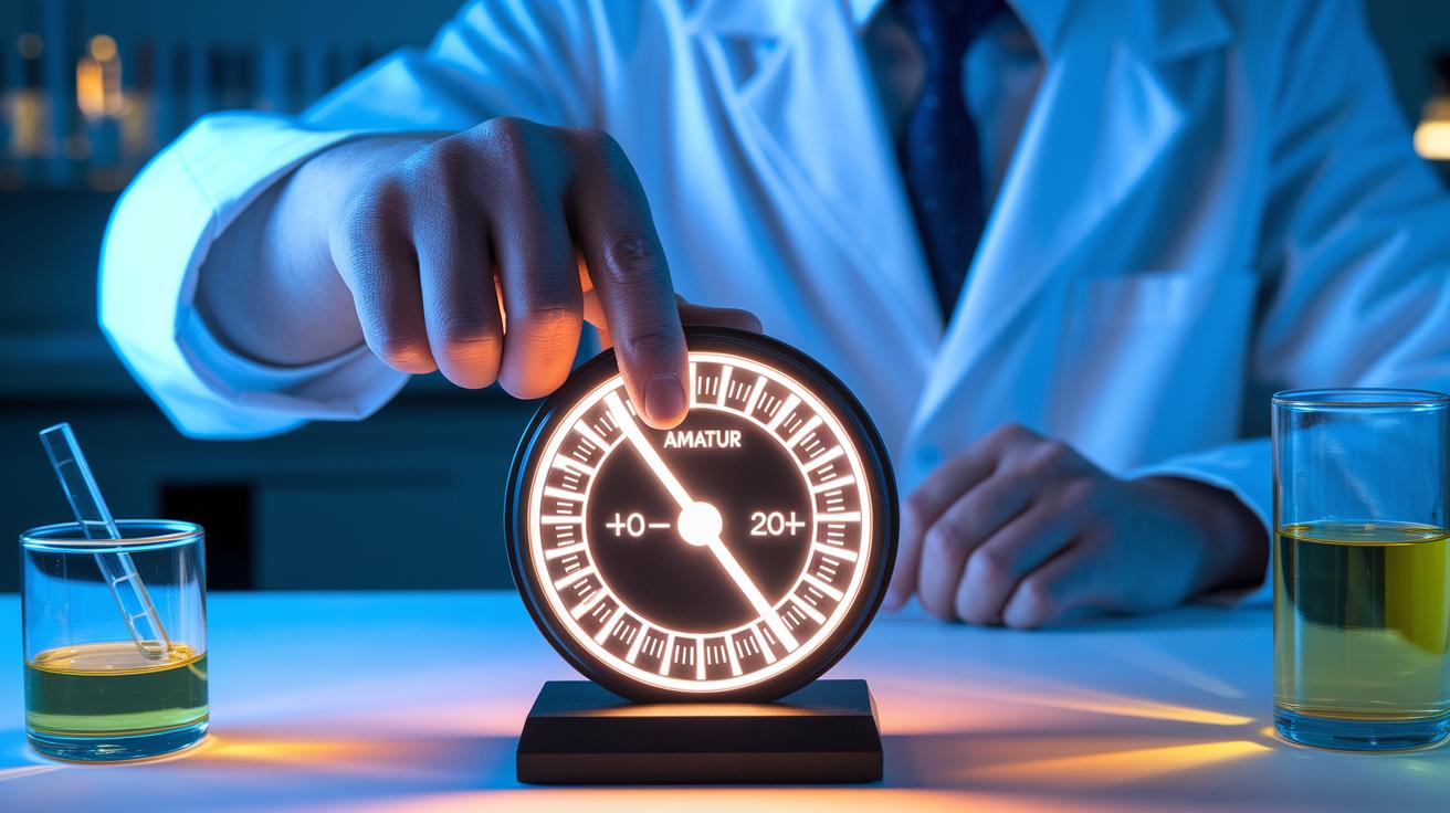
Imagine turning a dial on a quantum device so slowly that the system hardly ever jumps to a higher energy level. This gradual adjustment means the system carefully follows the path laid out by its changing settings. The whole idea is supported by a key rule in quantum mechanics, the adiabatic theorem, which says that if you let the change happen slowly enough, the system is almost certain to remain in its lowest energy state. This smooth, gentle change sets adiabatic quantum optimization apart from other methods that use quick, step-by-step operations, making it a clever way to solve challenging computational problems.
The Adiabatic Theorem as the Theoretical Framework
In quantum mechanics, the adiabatic theorem tells us that if you change a system’s Hamiltonian slowly enough compared to ℏ divided by the energy gap (Δ), the system stays in its current state. It’s a bit like carefully coaxing a sleeping cat so you don’t startle it.
When the energy gap becomes really small, especially around what are known as avoided crossings, you need to give the system plenty of time. In these cases, the evolution time (T) should be much longer than ℏ divided by Δ². Imagine slowly turning the dial on a quantum gadget; if you speed through when the gap is narrow, you might trigger something called a Landau–Zener transition, which can knock the system out of its calm, ground state.
Simple proofs of this idea use time-dependent perturbation theory (a method for looking at how small changes affect a system) and compare it with the Born–Oppenheimer approach (which separates the movement of heavy and light particles). These studies support the idea that if you move slowly, the system's ground state remains steady. Here are the key points:
| Key Point | Description |
|---|---|
| Slow Change | If the Hamiltonian changes slowly compared to ℏ/Δ, the system stays in its ground state. |
| Small Energy Gap | When Δ is very small, T must be much larger than ℏ/Δ² to avoid transitions. |
| Support from Theory | Time-dependent perturbation theory backs up these conditions. |
Think of slow evolution like carefully stepping down a staircase; rush it, and you might stumble into an excited state, but a measured pace keeps you safely on track. This idea not only forms the mathematical basis for adiabatic quantum computing but also sets the practical limits on how fast a quantum system can work reliably.
Practical Algorithmic Implementations and Simulation Steps
When you write code for an adiabatic algorithm, you’re making a digital version of a quantum system (a tiny world following special rules) that slowly changes from a starting setup (H_i) to a final one (H_f) that holds the answer. In these simulations, we chop up both positions and speeds (momentum) into neat pieces so we can use Schrödinger’s equation (the recipe for quantum behavior) with simple units (where ℏ = 1). For example, if you ease the potential from V_i to V_T slowly, more than 90% of the system sticks with the lowest energy. But if you speed it up (like using T/3), the system gets too excited and jumps to higher energy levels.
When coding this in a Python setup such as Jupyter Notebook, picking the right simulation time T and time step Δt is key. A long T lets the system adjust smoothly, like slowly stirring a thick smoothie. On the other hand, rushing the process means the system can’t follow its intended energy steps, and you see that as the energy spreading out into other states.
Let’s break it down into five simple steps:
- Define H_i and H_f in discrete form
- Choose a simulation time T and a small time step Δt
- Rewrite Schrödinger’s equation using a method that approximates changes (finite-difference method)
- Run the evolution operator U(t) from 0 to T
- Check how much it matches the ground state at every moment
These steps make sure your code captures the slow, steady changes of a quantum system. Think of it as taking tiny, careful steps on a slippery path so you don’t lose balance. Working through these simulations not only deepens your grasp on the adiabatic approach in quantum mechanics but also ties big theoretical ideas to real, hands-on coding practice.
By fine-tuning these settings, you gain a clear view of how this quantum trick, using the adiabatic approximation, translates into practical, simulation-based solutions for real-world challenges.
Contrasting Adiabatic Quantum Computing with Gate-Based and Annealing Models

Gate-based quantum computers use separate, simple steps, like adding one building block after another, to get their work done. In contrast, adiabatic quantum computing (AQC) slowly shifts a smooth energy setup (known as a continuous Hamiltonian) from an easy starting point to a final state that holds the answer. It’s a bit like gently turning a dimmer switch until you reach just the right light. Meanwhile, quantum annealing (QA) mixes in a few quick, less smooth changes along with a bit of heat-related settling (thermal relaxation). This often means it runs faster, but it might not hit the exact answer as precisely as AQC does. If you’re curious about more digital details, have a look at How quantum computers work.
Every method comes with its own pros and cons. AQC aims to capture the exact lowest-energy state (or ground state) for superb precision, but it takes more time because of its slow, careful process. Gate-based computers offer flexibility by working with short, precise bursts, though they often need complex fixes when errors pop up. On the other hand, QA does a bit of a trade-off, it gives up some precision in exchange for speed, which can be just right when near-perfect answers are acceptable.
Here is a quick comparison:
| Feature | Description |
|---|---|
| Runtime | AQC works more slowly due to its gradual approach; gate-based and QA methods run faster. |
| Error Resilience | AQC’s smooth process helps it avoid sudden mistakes, while gate-based systems often need extra error fixes. |
| Solution Precision | AQC is built to get the exact ground state, whereas QA usually offers answers that are nearly perfect. |
| Hardware Complexity | Gate-based computers depend on detailed circuit design, while AQC uses a more continuous, gradual change. |
| Noise Tolerance | AQC often handles disruptions better, thanks to its steady evolution, compared to the quick pulses in gate-based methods. |
| Typical Applications | AQC is great for tough optimization challenges, and gate-based plus QA setups are versatile for many quantum tasks. |
Real-World Use Cases for Adiabatic Quantum Approaches
Adiabatic quantum computing is finding its place in many areas. Imagine a process where a system slowly shifts from a simple starting point to a final state that holds the best answer, that’s how this approach solves tricky puzzles like the Traveling Salesman Problem, Max-Cut, and Graph Partitioning. Think of it as gently guiding a maze until the exit is clear.
In the world of machine learning, this method helps refine models, much like carefully placing one puzzle piece after another until you see the full picture. It works by reducing errors in techniques like support vector machines (a type of model that separates data into groups) and enhancing clustering methods so data naturally falls into place.
Materials science also gets a big boost from adiabatic quantum methods. Researchers use these techniques to find the lowest energy states or “ground states” in chemical and physical systems, revealing the most stable molecular layouts. Even finance benefits, by methodically checking different market scenarios, portfolio optimization, risk analysis, and even pricing options for derivatives become more robust.
| Area | Application |
|---|---|
| Combinatorial Optimization | Solves tough puzzles like the Traveling Salesman Problem |
| Machine Learning | Improves loss functions and clustering methods |
| Materials Science | Identifies stable ground states in complex systems |
| Finance | Enhances portfolio optimization, risk analysis, and pricing |
By gradually encoding states, using tools like quantum computing qubits (tiny bits that represent data in quantum systems), adiabatic quantum computing is steadily transforming how we tackle optimization across many fields. Have you ever thought about how a slow, careful change can lead to precise and powerful solutions?
Challenges, Limitations, and Emerging Solutions in Adiabatic Systems

Adiabatic quantum computing faces big hurdles as we try to scale it up. One major issue is the tiny energy gaps (small differences in energy) seen in large-scale problems. These small gaps force the evolution time T to grow roughly like ℏ (Planck’s constant, a tiny fixed number in quantum physics) divided by Δ². Because the process takes so long, the system is more likely to be disturbed by decoherence (loss of quantum information) and thermal noise (random heat fluctuations) that can cause unwanted glitches.
In practice, getting the shape of the Hamiltonian pulses just right is crucial, imagine slowly turning a delicate knob to keep an instrument perfectly tuned. This strict level of control makes building the necessary hardware both expensive and hard to manage.
Researchers are busy tackling these challenges with fresh error mitigation strategies (methods to reduce mistakes) and sturdier system designs. Even though adiabatic systems need less error correction work compared to traditional gate-based models, there’s still plenty of room for improvement. New solutions include advanced control electronics, smarter materials, and innovative pulse shaping techniques that help maintain accuracy even with narrow energy gaps.
Some scientists are even exploring hybrid methods that blend smooth adiabatic evolution with digital quantum elements, which could ease the demands for extreme precision. Overall, these efforts show a vibrant research scene focused on making adiabatic quantum devices more resilient and energy efficient as we move toward practical, large-scale quantum computing.
adiabatic quantum computing: Fascinating Concepts & Trends
Researchers are mixing two exciting ideas in quantum computing. They’re exploring ways to blend smooth, continuous quantum changes with step-by-step, digital controls. In simple terms, scientists are trying out new hybrid methods (like QAOA, which is a kind of algorithm that uses both approaches) so that the computer parts stay at their lowest energy state, even when tackling really tough puzzles.
Early tests are looking good. Small experiments show that these methods could soon lead to quantum processors that grow bigger and better over time. Researchers are even designing special techniques for machine learning and building in error fixes. In short, by combining these ideas, we might soon see quantum computers that can solve real-life challenges more accurately and efficiently.
Final Words
In the action, we explored how a slow Hamiltonian evolution leads to reliable outcomes, breaking down the core ideas of maintaining a system’s ground state and simulating each step. We touched on building and testing these algorithms, compared them with other quantum models, and showcased practical use cases.
The discussion wraps up with insights into ongoing research trends and improvements, leaving us inspired about the potential of adiabatic quantum computing.
FAQ
What is adiabatic quantum computing?
Adiabatic quantum computing uses a slow, continuous change in system conditions (Hamiltonian evolution) to keep the quantum system in its lowest energy state, enabling it to encode and solve complex problems.
How powerful is adiabatic quantum computation?
Adiabatic quantum computation can theoretically match the problem-solving power of standard quantum computing, although its effectiveness hinges on precise control and the size of the energy gap between states.
What is the quantum adiabatic theorem?
The quantum adiabatic theorem explains that a system remains in its instantaneous ground state if its governing parameters change slowly enough compared to a rate determined by the smallest energy gap between the ground and excited states.
Is adiabatic quantum computing universal?
Adiabatic quantum computing is considered universal since it can, in theory, solve the same range of problems as standard quantum computing, but it typically demands longer runtimes to maintain its exact ground-state evolution.
How does adiabatic quantum computing differ from quantum annealing?
Adiabatic quantum computing relies on strictly slow state evolution to stay in the ground state, while quantum annealing allows faster transitions and thermal effects to find approximate solutions more quickly.